Tutorial

 

With Simple ML for Sheets, also referred to as Simple ML, everyone can use Machine Learning (ML) in Google Sheets without knowing ML, without coding, and without sharing data with third parties.

This tutorial takes you through the steps of using Simple ML for Sheets to solve three exercises: Predicting missing values (task 1), identifying abnormal values (task 2), and training / evaluating & understanding a model manually (task 3).

Prerequisites

This tutorial is easier to follow if you are familiar with Google Sheets. For example, make sure you know the basics like how to select columns or set a cell value.

What you’ll learn

• How to install Simple ML for Sheets.

• How to use Simple ML to predict missing values in your data.

• How to spot abnormal values in your data.

• (Advanced) How to train/evaluate/interpret and productionize a model.

Install Simple ML for Sheets

First, install Simple for Sheets.

1. Go to Simple ML for Sheets in Google’s Marketplace and click the Install button.

   

2. Grant permissions.

   Why?: Simple ML stores your machine learning models in your Google Drive in the simple_ml_for_sheets directory.

3. We assembled a spreadsheet with example data. Open and make a copy of this spreadsheet.

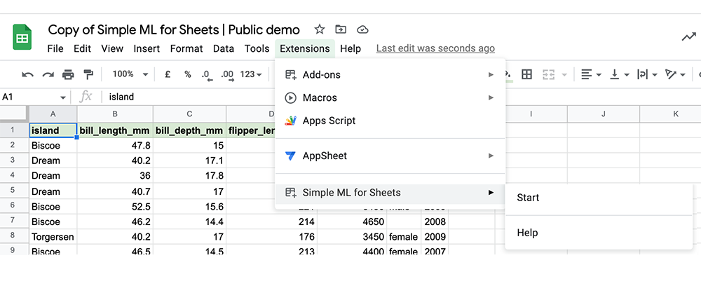
4. In the Google Sheets spreadsheet, check that Simple ML is visible in the Extensions menu. If the addon is not visible, wait a few seconds and refresh the page. The addon can take a minute to appear after being installed.

   

Task 1: Predict missing values

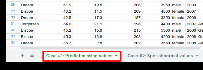
Open the first tab called “Case #1: Predict missing value”.

Scenario

You are studying a colony of penguins in Antarctica. This colony is composed of three penguin species: Chinstrap, Gentoo, and Adelie.

Image by Allison Horst

You are studying the differences between these species. Your colleague has collected physiological measurements (such as size and weight) of approximately 300 penguins. However, they got distracted in the process, and they forgot to note the species of 30 penguins.

You want to use Simple ML to recover the species of those 30 penguins.

1. Scroll up and down through the data.

   This sheet contains data about penguins. Each row represents a penguin while each column represents a physiological aspect of the penguin.

   The last column called species represents the species of the animals. The species is missing for the first 30 rows.

2. Open Simple ML. In the menu, click on Extensions > Simple ML for Sheets > Start.

   

3. Wait for the Simple ML side panel to appear (It might take a few seconds).

   

Predict Missing values

Once Simple ML is loaded, you can use it to predict missing values.

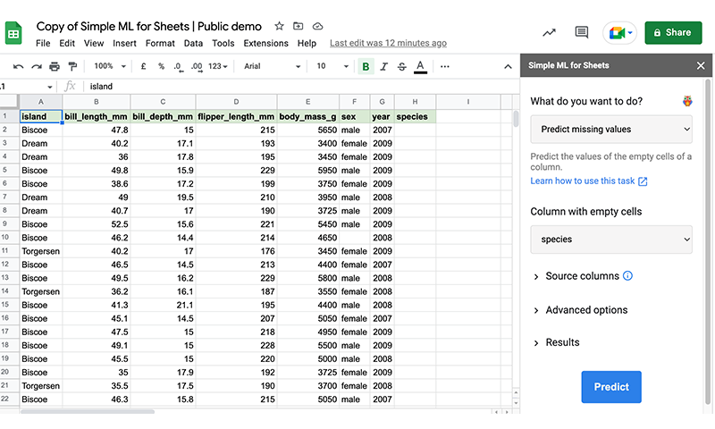
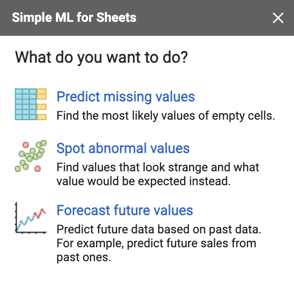
1. First, notice that some rows are missing values in Column H, species.

2. In the Simple ML for Sheets side panel, make sure that the field What do you want to do? is set to Predict missing values.

   

3. In the “Column with empty cells” section, select the column species. This is the column that contains the missing values you want to predict.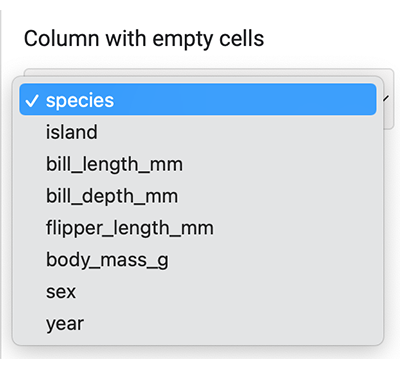

   

4. Click the Predict button.

   

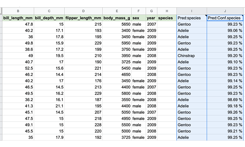
After a few seconds, two new columns appear:

• Pred:species are the predicted values for the species column.

• Pred:Conf.species are the confidences of the predicted value. In other words, this column indicates how confident the model is about the predictions in the column Pred:species. Confidence is a percentage between 0% and 100%, where 100% means that the model is sure of its prediction.

Some questions for you

Look at the predicted values of species. Do they look reasonable to you?

Feel free to experiment with predicting missing values in other columns.

For the ML experts

Behind the scenes, the task Predict missing value collects rows with species values and uses those rows to train a model. This model is then applied to the rows with missing species values. The model is available in the Manage models task and in the folder simple_ml_for_sheets of your Google Drive.

Task 2: Spot abnormal values

Open the first tab called “Case #2: Spot abnormal values.”.

This sheet contains physiological data about abalones (a type of marine snail). Like in task #1, each row represents an animal while each column represents a physiological aspect of the animals.

Scientists can tell the age of an abalone from the number of rings in its shell like you can tell the age of a tree by the number of rings in its trunk. This dataset contains records for around 4’000 abalones. In this task, the goal is to look for abnormalities in the number of rings in abalones.

Compute the abnormality score

1. Select the Case #2: Spot abnormal values tab

2. If Simple ML is not already open, open it Extension > Simple ML > Start

3. Under What do you want to do? select Spot abnormal values.

4. Select the column you want to analyze. In this case, it’s the Rings column.

5. Click Spot abnormal values.

After a few seconds, two new columns are created on the right side of your data: Pred:Abnormality:Rings and Pred:Mostlikely:Rings.

• Pred:Abnormality:Rings are the “abnormality scores” ranging from 0 (most normal) to 1 (most abnormal). They tell how similar to other values each row is.

• Pred:MostLikely are the most likely predicted values for the selected column. In some cases, this will be the same as the existing value, in other cases, the predicted value will be different than the existing value.

Look for the most abnormal rows

It is sometimes interesting to look at the most “abnormal” values by sorting the rows according to the Pred:Abnormality column. Abnormal values are sometimes indicative of an error in the data or a normal aspect of the dataset.

Note

While counterintuitive, in many situations it is normal to have abnormal values, and it is abnormal for all the rows to behave the same. This means that a value with a high abnormality score does not necessarily mean that the value has errors or was misreported.

1. Select the column header for the Pred:Abnormality:Rings column by clicking on the “Pred:Abnormality:Rings” text.

2. In the Data menu, click Sort Sheet > Sort Sheet By Column J (Z to A). Make sure to choose Z to A otherwise the rows with values greater than 0 in that column will be at the bottom of the sheet.

Once the sheet is sorted with the highest abnormality values at the top, look at the first row/animal: The first abalone has 29 rings, which is a lot. But the model thinks that this abalone should only have 12 or 13 rings. In other words, this abalone is very old, but it looks much younger.

Look at other columns

Continue to explore abnormal values for other columns (and change some values manually if you like).

For the ML experts

Under the hood, ten different models are trained using a 10-fold cross-validation protocol. Each value in the target column is then compared to the prediction of the corresponding model in the cross-validation. If the existing value and the predicted value do not match, the row is considered abnormal. For details, check the task documentation.

You can also remove some of the features from Source Columns or change the learning algorithm: By default Simple ML uses a Gradient Boosted Trees learning algorithm.

Before going deeper

Congratulations to you if you reached this point in the tutorial. You now can use Machine Learning to solve real problems. We invite you to put this new knowledge to practice on your data.

Like riding a bike, it might seem hard at first, but it becomes easy quickly: You will see opportunities for ML everywhere in no time 😀.

This marks the end of the beginner tutorial. The next section shows how ML experts can do standard ML work with Simple ML. This section is written for people who are already familiar with machine learning but we encourage everybody to read it.

If you want to learn Machine Learning, you should check out the Google Machine Learning class and use Simple ML to practice.

Task 3: How to train/evaluate/interpret and productionize a model

You have learned how to use Simple ML to predict missing values and spot abnormalities in data.

Underneath, Simple ML has created several machine learning models: One model was trained in task #1, and ten models were trained but not saved in task #2. However, it is sometimes necessary to create, evaluate and use ML models manually. In task #3, you will see how to train, evaluate, analyze and interpret, and finally export an ML model into a Colab.

Note

Colab is a popular platform to write programs using the Python programming language to do ML learning work. In this example, the model will be trained with Simple ML for Sheets and then exported to collab to run inference.

Training a model

The first step is to train your ML model. The tabs “Case #3: Training dataset” and “Case #3: Evaluation dataset” contains respectively a training and testing dataset that you will use to train and evaluate a model.

1. Select the “Case #3: Training dataset” tab.

2. Under What do you want to do? select Train a model.

3. Name your model “My first model”.

4. Under Label select species. The model will try to predict the species column.

5. For now, do not change the source columns or the advanced options.

6. Click Train.

After a few seconds, the model is trained and ready to be used. Press the Close button.

Analyse & Interpret the model

It is sometimes interesting to understand what is inside a model. Let’s take a look.

1. Under What do you want to do? select Understand a model.

2. Under Models select the model you just trained called “My Model”.

3. Check the box Include sheet data.

4. Click Understand.

After a few seconds, the model understanding window appears.

In the Summary tab, you can see information about the input features of the model.

In the Quality tab, you can see evaluation metrics about the model. In this case, the evaluation was computed on a validation dataset extracted automatically from the training dataset. Different learning algorithms (in the “advanced options” section) might behave differently.

In the Dataset tab, you can see details about the input features of the model.

In the Variable importance tab, you can see how each feature impacts the model. For example, the feature variable importance MEAN_DECREASE_IN_ACCURACY indicate how much the quality of the model would “drop” if the feature was removed. The features with the highest feature importance are the most important to the model.

In the Predictions tab, you can see how the prediction of the model is impacted by different feature values.

Finally, in the Plot model tab, you can see a representation of the model. Note that only “Decision Tree” models are plotted (to be selected in the “advanced options” when training the model).

Evaluate the model

Measuring the quality of a model on a test set (also called “hold-out set”) is critical for measuring the overfitting of the model.

Note

During training, a validation dataset is automatically extracted from the training dataset to control the training. The evaluation of the validation dataset is present in the Model Understanding window shown in the previous step. In the current step, the model will be evaluated manually on a new dataset.

1. Select the “Case #3: Evaluation dataset” tab.

2. Under What do you want to do? select Evaluate a model.

3. Under Models select the model you just trained called “My Model”.

4. Click Evaluate.

After a few seconds, the model evaluation window appears. Don’t hesitate to scroll to see evaluation plots.

Export model

For the last step of this tutorial, you will export the model to a Colab.

1. Select the “Case #3: Evaluation dataset” tab.

2. Under What do you want to do? select Export a model.

3. Under Models select the model you just trained called “My Model”.

4. Under Destination select Colab (External).

5. Click Export.

After a few seconds, a window showing a snippet of python code appears. You can paste and run this code in a new Colab document. You will see the predictions of the model.

Note

Model predictions can also be computed in Sheets with Simple ML with the Make predictions with a model task.

Learn More

Congratulations! You have learned how to use Simple ML for Sheets to predict missing values and spot abnormalities in your data, and you have briefly looked at some of the advanced options available for working with models that Simple ML creates.

You can do much more with Simple ML than this introductory tutorial covers.

For more details, see:

• Simple ML for Sheets documentation

• FAQ

If you’re interested in learning about the Decision Forests technology that underlies Simple ML, see the Decision Forests course at developers.google.com/machine-learning/decision-forests.